8. Writing Optimizers in NC


When you press the Run button in the NC window, NC will run the model that you have specified. For example, a simple 20m dipole model shown below




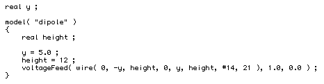
Notice that we have declared y to be a global variable. There is a reason for this. This allows us to later set the value of y from a different place than from inside the model itself.


control Function

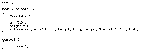
In addition to the model function, NC has a second special function called control. If your program includes a control function, the Run button will run the control function rather than the model function.

In turn, NC also provides a runModel function call which allows you to run the model from a control function. Each pass through the model function will cause NEC-2 or NEC-4 to be executed.

The following program will produce the same results as the example above since Run will execute the code in control. The runModel in the control function will in turn run the model indirectly.




Since y is a global variable, it allows us to set its value from the control function, viz:




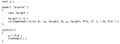
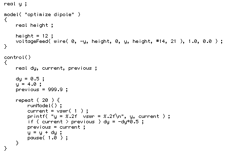
Notice that we can now write a program such as the following:





After the repeat loop has completed, this is what the NC Output Console looks like:



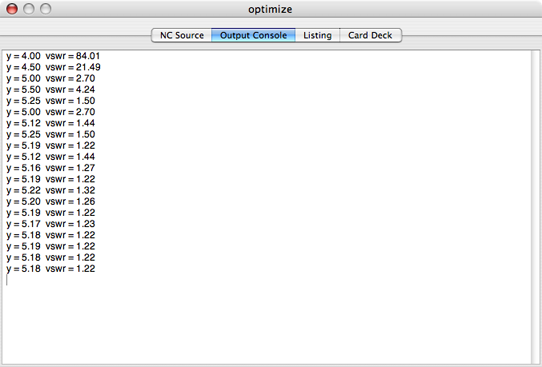
Each printf statement in the repeat loop has generated a line of output in the Console.

Notice that after repeatedly adjusting the value for y, the vswr has converged to about 1.22:1.

Let us inspect the control function in greater detail.

The control function starts by initializing the y increment (dy) to .5, and the value of y itself to 4.0. It also initializes a variable called previous to a large value.

The repeat loop then runs the model with the runModel statement. The model will make use of the y value that is set by the control loop. When runModel returns, the repeat loop inspects the value of a function called vswr to extract the VSWR for the first (and only) feed point for the model. It also prints out both the value for y and the current value of the VSWR.

We then compare this current VSWR value against the previous VSWR value. If the VSWR had increased instead of continuing to decrease, we make the guess that we have overshot the optimal value for y. We therefore change the sign of the y increment value and also reduce the magnitude of the y steps by half. We then update the "previous" VSWR value and change y to the next estimate.

As a result, the loop will cause the y value to adapt to a value that minimizes the VSWR, as can be seen in the output window above. By inspecting the end value for y, we see that it has converged to a value of 5.18 meters.


Functions and Variables to Access NEC-2 Output

Notice in the above that we used a function named vswr( 1 ) to access the VSWR value of the model. The argument 1 indicates that we are looking for the VSWR of the first feed point. For a model that has more than one feed point, you can use vswr( 2 ), vswr( 3 ), etc to inspect the VSWR of the other feed points. The function vswr is only accessible from the control function. It is not visible from the model itself, since VSWR is the result of running the model.

The following functions can be used in a control function to inspect the output of a model:


vswr( feed )


feedpointImpedanceReal( feed )


feedpointImpedanceImaginary( feed )


feedpointVoltageReal( feed )


feedpointVoltageImaginary( feed )


feedpointCurrentReal( feed )


feedpointCurrentImaginary( feed )



There are also some special variables that you can use to access NEC-2 output values:


maxGain


azimuthAngleAtMaxGain


elevationAngleAtMaxGain


directivity


frontToBackRatio


frontToRearRatio



In addition, there is a function that you can call to ask NEC-2 to use double precision or quad precision computation (the default is double precision):


useQuadPrecision( state )